Introduction
Human Skin Detection in Color Images
Thesis Overview
See full thesisThe purpose of the thesis is to present a review of the human skin detection datasets and approaches of the state of the art, and then perform a comparative in-depth analysis of the most relevant methods on different databases.
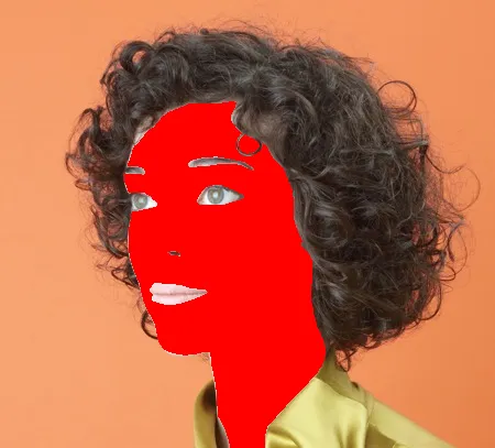
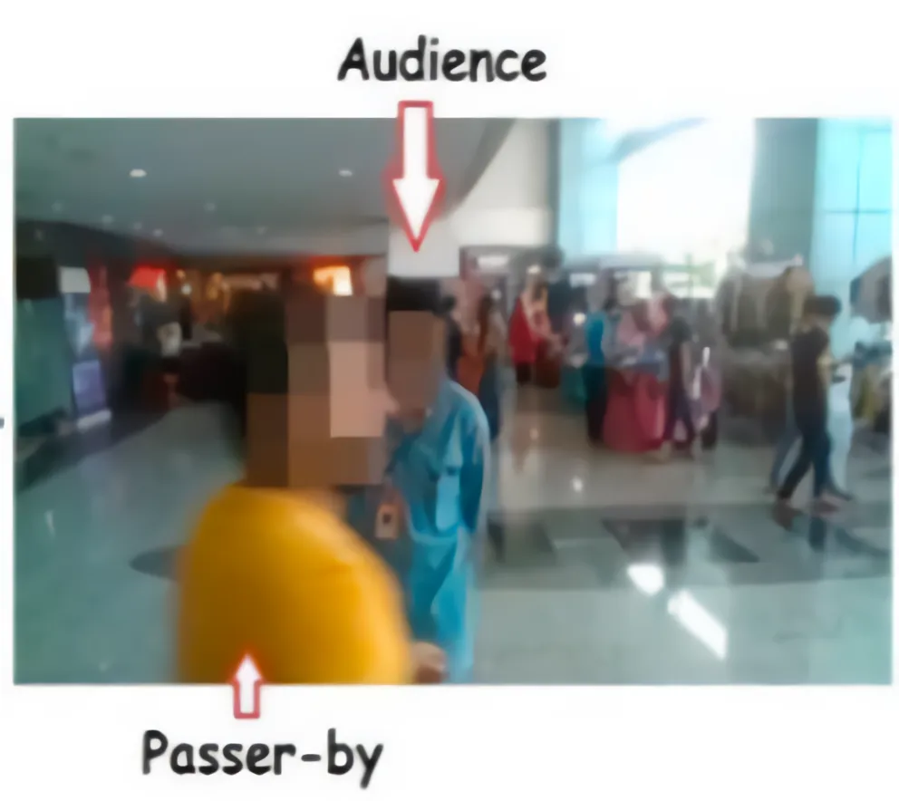
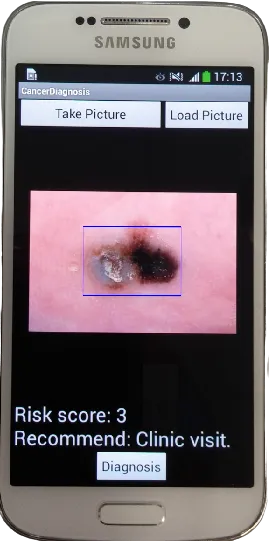
Skin detection is the process of discriminating skin and non-skin pixels. It is quite a challenging process because of the large color diversity that objects and human skin can assume, and scene properties such as lighting and background.
Limitations
- Materials with skin-like colors
- Wide range of skin tones
- Illumination
- Cameras color science
Methodological Approach

Taxonomy
Skin detection is a binary classification problem: the pixels of an image must be divided between skin and non-skin classes.
One of several ways to categorize methods is to group them according to how the pixel classification is done.
Rule-based
classifier
Thresholding approaches use plain rules to classify each pixel as either skin or non-skin. An example is the following.
A given (Y,Cb,Cr) pixel is a skin pixel if 133<=Cr<=173 and 77<=Cb<=127
Investigated Methods
Thresholding, Statistical, and Deep Learning have been the chosen approaches.
The first to demonstrate whether simple rules can achieve powerful results; and the latter two to compare how differently the models behave and generalize, and whether the capabilities of a CNN to extract semantic features can give an advantage.
Algorithm Overview
- Input image RGB to YCbCr
- Crmax Cbmin computation
- Pixel-wise computation of the correlation rules parameters
- Pixel-wise correlation rules check
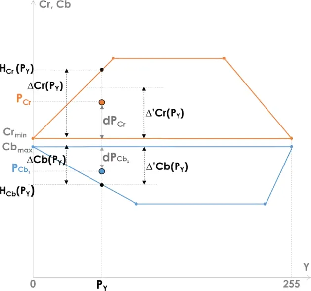
Brancati et al. 2017 [4]
The skin pixels clusters assume a trapezoidal shape in the YCb and YCr color subspaces. Moreover, the shape and size of the trapezium vary according to many factors, such as the illumination conditions. In high illumination conditions, the base of the trapezium results larger.
Besides, the chrominance components of a skin pixel P with coordinates (PY, PCb, PCr) in the YCbCr space exhibit the following behavior: the further is the (PY, PCr) point from the longer base of the trapezium in the YCr subspace, the further is the (PY, PCb) point from the longer base of the trapezium in the YCb subspace, and vice versa.
The aforementioned observations are the base of the method: it tries to define image-specific trapeziums in the YCb and YCr color subspaces and then verifies that the correlation rules between the two subspaces reflect the inversely proportional behavior of the chrominance components.
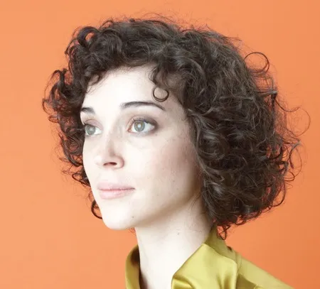
![The accumulation points may indicate a feature to extract The resulting 3D histogram from the image featuring the girl with the orange background: each pixel is taken from the original image and stored at the coordinates [R,G,B] of the histogram. The visualization of the resulting three-dimensional histogram features some accumulation points which may indicate some interesting features to extract from the image. For example the plain orange background can easily be identified as it represents lot of pixels with low variance.](/skin-detection-io/assets/images/3d_hist-501aa114be85f501ef7919f617c87770.webp)
Example of an image's 3D Histogram
Train
- Initialize the skin and non-skin 3D histograms
- Pick (image, mask) from the training set
- Loop every RGB pixel from image
- By checking its mask, the pixel its either skin or non-skin. Add +1 to the relative histogram count at coordinates [r,g,b]
- Return to step 2 until there are images
Predict
- Define classifying threshold Θ
- Loop every RGB pixel from input image
- Calculate RGB probability of being skin
- If skin probability > Θ, it is classified as skin
The data is modeled with two 3D histograms representing the probabilities of skin and non-skin classes, and classification is performed via probability calculus by measuring the probability P of each rgb pixel to belong to the skin class:

where s[rgb] is the pixel count contained in bin rgb of the skin histogram and n[rgb] is the equivalent count from the non-skin histogram.
A particular rgb value is labeled skin if:

where 0 ≤ Θ ≤ 1 is a threshold value that can be adjusted to trade-off between true positives and false positives.
Workflow
- Pre-process input image: resize (512×512)px, padding
- Extract features in the contracting pathway via convolutions and down-sampling: the spatial information is lost while advanced features are learnt
- Try to retrieve spatial information through up-sampling in the expansive pathway and direct concatenations of dense blocks coming from the contracting pathway
- Provide a final classification map
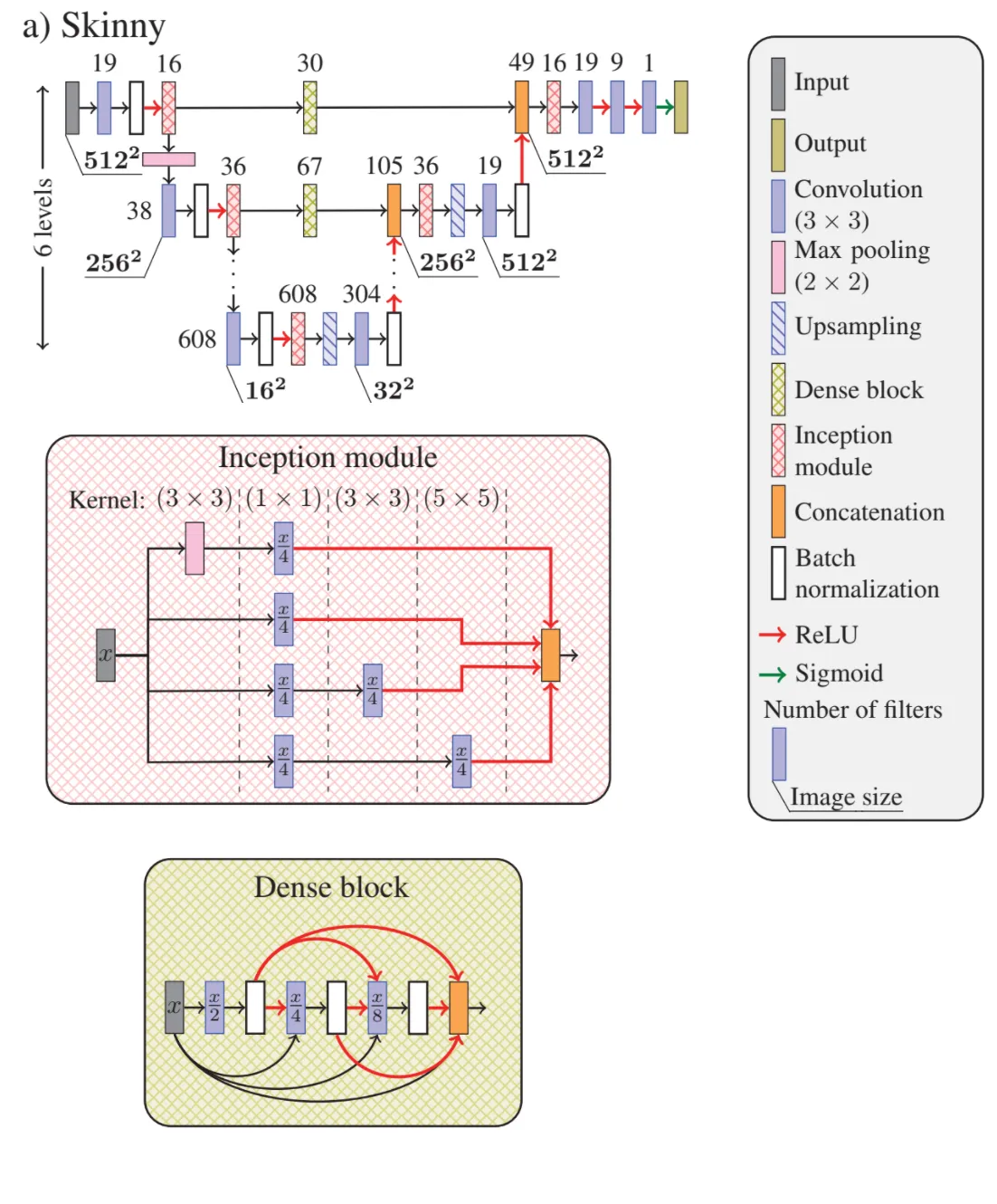
Tarasiewicz et al. 2020 [5]
The Skinny network consists of a modified U-Net incorporating dense blocks and inception modules to benefit from a wider spatial context.
The network is called "U-Net" because of its shape: there is a contracting path which tries to extract increasingly complex features as it goes deeper, and an expanding path which tries to retreive the lost spatial information during the feature extraction
An additional deep level is appended to the original U-Net model, to better capture large-scale contextual features in the deepest part of the network. The features extracted in the contracting path propagate to the corresponding expansive levels through the dense blocks.
The original U-Net convolutional layers are replaced with the inception modules: before each max-pooling layer, in the contracting path, and after concatenating features, in the expanding path. Thanks to these architectural choices, Skinny benefits from a wider pixel context.


The salient content size varies between images. Inception module combines multiple kernels with different sizes for content adaptation.

Dense block layers are connected in a way that each one receives feature maps from all preceding layers and passes its feature maps to all subsequent layers.
Datasets
Image databases are essential for developing skin detectors. Over the years, new databases keep getting published, but there are still some limitations on their reliability:
- Unbalanced classesMay cause some metrics to give overoptimistic estimations [6]
- Number of images
- Image quality
- Ground truth quality
- Lack of additional dataThis kind of data may be extremely useful in some applications:
- Lighting conditions
- Background complexity
- Number of subjects
- Featured skin tones
- Indoor or outdoor scenery
ECU, HGR, and Schmugge are the chosen datasets for this work as they describe a good overall score considering popularity, diversity, size, and the previously mentioned issues.
Here are the common datasets used in Skin Detection.
| Name | Year | Images | Shot Type | Skin Tones |
|---|---|---|---|---|
| abd-skin | 2019 | 1400 | abdomen | african, indian, hispanic, caucasian, asian |
| HGR | 2014 | 1558 | hand | - |
| SFA | 2013 | 1118 | face | asian, caucasian, african |
| VPU | 2013 | 285 | full body | - |
| Pratheepan | 2012 | 78 | full body | - |
| Schmugge | 2007 | 845 | face | labels: light, medium, dark |
| ECU | 2005 | 3998 | full body | whitish, brownish, yellowish, and darkish |
| TDSD | 2004 | 555 | full body | different ethnic groups |
VPU [11] as for Video Processing & Understanding Lab, consists of 285 images taken from five different public datasets for human activity recognition. The size of the pictures is constant between the images of the same origin. The dataset provides native train and test splits. It can also be referred to as VDM.
Results
For example, with ECU as the dataset, it means that the skin detector is eventually trained using the training set of ECU, and then tested on the test set of ECU.
In single evaluations, methods are eventually trained on the training set (in the case of trainable methods), and then predictions are performed on the test set.
For example, with ECU as the training dataset and HGR as the testing dataset, it means that the skin detector is trained using the training set of ECU, and then tested on all the HGR dataset.
In cross evaluations, only trainable approaches are analyzed. Detectors are trained on the training set, and then predictions are performed on all the images of every other datasets.
The expression HGR on ECU describes the situation in which the evaluation is performed by using HGR as the training set and ECU as the test set.
Initially, the metrics are measured for all the instances, then the average and population standard deviation for each metric are computed.
Single Dataset

Where PR is Precision, RE is Recall, and SP is Specificity; and (1,1,1) the ideal ground truth.
| Method \ Database | ECU | HGR | SCHMUGGE | |
|---|---|---|---|---|
| F1 | U-Net | 0.9133 ± 0.08 | 0.9848 ± 0.02 | 0.6121 ± 0.45 |
| Statistical | 0.6980 ± 0.22 | 0.9000 ± 0.15 | 0.5098 ± 0.39 | |
| Thresholding | 0.6356 ± 0.24 | 0.7362 ± 0.27 | 0.4280 ± 0.34 | |
| IoU | U-Net | 0.8489 ± 0.12 | 0.9705 ± 0.03 | 0.5850 ± 0.44 |
| Statistical | 0.5751 ± 0.23 | 0.8434 ± 0.19 | 0.4303 ± 0.34 | |
| Thresholding | 0.5088 ± 0.25 | 0.6467 ± 0.30 | 0.3323 ± 0.28 | |
| Dprs | U-Net | 0.1333 ± 0.12 | 0.0251 ± 0.03 | 0.5520 ± 0.64 |
| Statistical | 0.4226 ± 0.27 | 0.1524 ± 0.19 | 0.7120 ± 0.54 | |
| Thresholding | 0.5340 ± 0.32 | 0.3936 ± 0.36 | 0.8148 ± 0.48 |
Schmugge appears to be the hardest dataset to classify, also presenting high standard deviations that can be attribuited to its diverse content, featuring different subjects, backgrounds, and lighting.
HGR seems to be the easier dataset to classify, which can be due to the relatively low diversity of subjects and backgrounds. In fact, learning approaches tend to have very high measurements.
In the ECU dataset, the results of Statistical and Thresholding are relatively close, while U-Net outperforms them by far.
U-Net beats its competitors in all the measurements, while Statistical comes always second.
NOT REPRESENTATIVE OF OVERALL PERFORMANCES!!
(for the skin detectors performance read the tables)
Instead their purpose is trying to highlight the strength and limitations of each skin detector by making a comparison.
Significant Outcomes
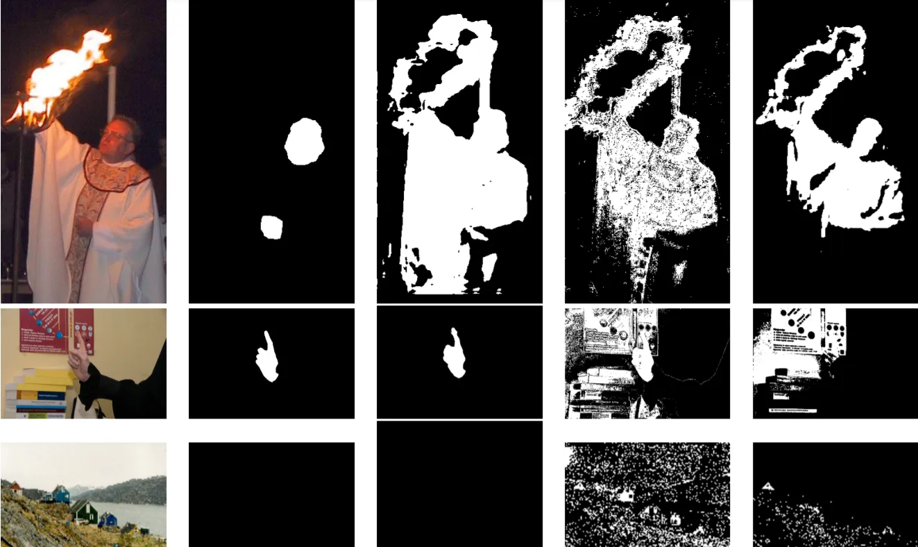
Skin detection results. (a) input image; (b) ground truth; (c) U-Net; (d) Statistical; (e) Thresholding
All approaches struggle on the first image as the lighting is really tricky. Even the U-Net describes a very bad classification, with a tremendous number of False Positives. Thresholding is the most restrictive on False Positives in this instance.
Color-based methods struggle on images without skin pixels and containing materials with skin-like color, with Statistical having a really high number of False Positives.
Cross Dataset
| Training | ECU | HGR | SCHMUGGE | ||||
|---|---|---|---|---|---|---|---|
| Testing | HGR | SCHMUGGE | ECU | SCHMUGGE | ECU | HGR | |
| F1 | U-Net | 0.9308 ± 0.11 | 0.4625 ± 0.41 | 0.7252 ± 0.20 | 0.2918 ± 0.31 | 0.6133 ± 0.21 | 0.8106 ± 0.19 |
| Statistical | 0.5577 ± 0.29 | 0.3319 ± 0.28 | 0.4279 ± 0.19 | 0.4000 ± 0.32 | 0.4638 ± 0.23 | 0.5060 ± 0.25 | |
| IoU | U-Net | 0.8851 ± 0.15 | 0.3986 ± 0.37 | 0.6038 ± 0.22 | 0.2168 ± 0.25 | 0.4754 ± 0.22 | 0.7191 ± 0.23 |
| Statistical | 0.4393 ± 0.27 | 0.2346 ± 0.21 | 0.2929 ± 0.17 | 0.2981 ± 0.24 | 0.3318 ± 0.20 | 0.3752 ± 0.22 | |
| Dprs | U-Net | 0.1098 ± 0.15 | 0.7570 ± 0.56 | 0.3913 ± 0.26 | 0.9695 ± 0.44 | 0.5537 ± 0.27 | 0.2846 ± 0.27 |
| Statistical | 0.5701 ± 0.29 | 1.0477 ± 0.35 | 0.8830 ± 0.23 | 1.0219 ± 0.42 | 0.7542 ± 0.30 | 0.6523 ± 0.27 | |
| F1 - IoU | U-Net | 0.0457 | 0.0639 | 0.1214 | 0.0750 | 0.1379 | 0.0915 |
| Statistical | 0.1184 | 0.0973 | 0.1350 | 0.1019 | 0.1320 | 0.1308 | |
Using HGR as the training set and predicting over Schmugge, Statistical outperforms U-Net, especially in the F1 score. While Statistical generally performs better than U-Net, it also includes a lot of False Positives, as the F1 - IoU and the Dprs metrics indicate. The latter is particularly bad in both cases, evidencing a big distance between the ideal ground truths and the predictions.
Training on Schmugge and predicting on ECU has the U-Net describing a slightly worse F1 - IoU, suggesting the presence of False Positives and False Negatives.
U-Net exceeds an F1 score of 80 in the case of Schmugge as the training set and HGR as the prediction set despite the size of the training set, which is not huge.
Apart from a few expections, U-Net still dominates.
Significant Outcomes
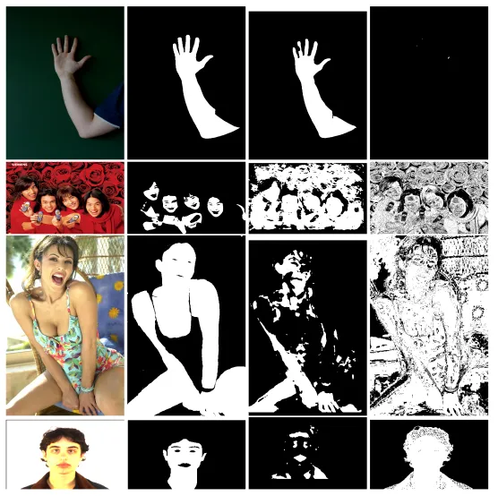
Skin detection results. (a) input image; (b) ground truth; (c) U-Net; (d) Statistical
It can be noticed how Statistical tends to exaggerate at classifying skin pixels in some cases, confirming the above intuitions on the statistical method having a lot of False Positives.
The third row (HGR on Schmugge) is part of the datasets combination in which Statistical outperforms U-Net. Statistical reports a lot of False Positives, but also a lot of True Positives, which U-Net struggles to identify. This kind of situation is why Dprs is better on U-Net despite F1 and IoU are worse: Dprs formula is partly driven by False Negatives (via Specificity), contrary to the other two metrics.
The last row (HGR on Schmugge) is also part of the same datasets combination and describes a similar situation: U-Net fails at labeling several skin pixels, especially on very lit regions, while Statistical overdoes it. This image represents the high complexity and diversity of the Schmugge content.
Single Skin Tone
| Method \ Database | DARK | MEDIUM | LIGHT | |
|---|---|---|---|---|
| F1 | U-Net | 0.9529 ± 0.00 | 0.9260 ± 0.15 | 0.9387 ± 0.12 |
| Statistical | 0.8123 ± 0.02 | 0.7634 ± 0.19 | 0.8001 ± 0.15 | |
| Thresholding | 0.2620 ± 0.14 | 0.6316 ± 0.20 | 0.6705 ± 0.14 | |
| IoU | U-Net | 0.9100 ± 0.01 | 0.8883 ± 0.18 | 0.9006 ± 0.14 |
| Statistical | 0.6844 ± 0.03 | 0.6432 ± 0.17 | 0.6870 ± 0.16 | |
| Thresholding | 0.1587 ± 0.10 | 0.4889 ± 0.19 | 0.5190 ± 0.14 | |
| Dprs | U-Net | 0.0720 ± 0.01 | 0.1078 ± 0.21 | 0.0926 ± 0.15 |
| Statistical | 0.3406 ± 0.05 | 0.3452 ± 0.23 | 0.3054 ± 0.20 | |
| Thresholding | 0.8548 ± 0.12 | 0.5155 ± 0.24 | 0.4787 ± 0.17 |
DARK presents an almost null standard deviation in learning approaches, indicating that the diversity of the images might not be very high.
The learning approaches have the highest difficulty at classifying the medium skin tones, which may be caused by the difficult scenarios featured in the sub-dataset, such as clay terrains, which have a skin-like color.
Thresholding struggles to classify dark skin tones, which may indicate that the skin clustering rules are leaving out the darker skin pixels.
U-Net beats its competitors in all the measurements, while Statistical comes always second.
Significant Outcomes
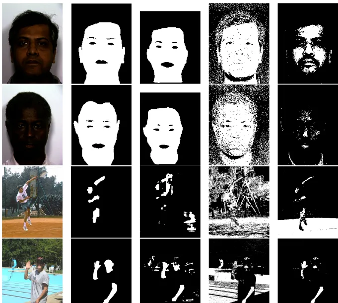
Skin detection results. (a) input image; (b) ground truth; (c) U-Net; (d) Statistical; (e) Thresholding
The first two rows depict darker skin tones. In both examples, it is possible to notice a pattern in the classification of each approach: U-Net produces almost ground truth-like predictions; Statistical tends to exaggerate on classifying skin pixels, but has an excellent number of True Positives; Thresholding seems to fail at classifying the darkest skin tones, but sometimes still manages to mark the inner regions of the face, which are often enough for describing the face shape.
The third row represents a tricky background with a clay terrain and medium skin tones. U-Net produces a very good prediction, while the other approaches include many False Positives. Statistical reports a tremendous number of False Positives, while Thresholding is deceived by the clay terrain and ruins its otherwise excellent classification.
In the last row, U-Net and Thresholding have very good predictions, with the former incorporating more False Positives, and the latter including more False Negatives. The statistical approach reports once again a huge number of False Positives.
Cross Skin Tone
| Training | DARK | MEDIUM | LIGHT | ||||
|---|---|---|---|---|---|---|---|
| Testing | MEDIUM | LIGHT | DARK | LIGHT | DARK | MEDIUM | |
| F1 | U-Net | 0.7300 ± 0.25 | 0.7262 ± 0.26 | 0.8447 ± 0.13 | 0.8904 ± 0.14 | 0.7660 ± 0.17 | 0.9229 ± 0.11 |
| Statistical | 0.7928 ± 0.11 | 0.7577 ± 0.12 | 0.5628 ± 0.14 | 0.7032 ± 0.14 | 0.5293 ± 0.20 | 0.7853 ± 0.11 | |
| IoU | U-Net | 0.6279 ± 0.27 | 0.6276 ± 0.28 | 0.7486 ± 0.15 | 0.8214 ± 0.16 | 0.6496 ± 0.21 | 0.8705 ± 0.13 |
| Statistical | 0.6668 ± 0.11 | 0.6229 ± 0.13 | 0.4042 ± 0.13 | 0.5571 ± 0.14 | 0.3852 ± 0.19 | 0.6574 ± 0.12 | |
| Dprs | U-Net | 0.3805 ± 0.33 | 0.3934 ± 0.34 | 0.2326 ± 0.17 | 0.1692 ± 0.18 | 0.3402 ± 0.21 | 0.1192 ± 0.16 |
| Statistical | 0.3481 ± 0.16 | 0.4679 ± 0.18 | 0.6802 ± 0.20 | 0.5376 ± 0.23 | 0.6361 ± 0.22 | 0.3199 ± 0.16 | |
| F1 - IoU | U-Net | 0.1021 | 0.0986 | 0.0961 | 0.0690 | 0.1164 | 0.0524 |
| Statistical | 0.1260 | 0.1348 | 0.1586 | 0.1461 | 0.1441 | 0.1279 | |
Using DARK as the training set and predicting over LIGHT, Statistical has better F1 but worse IoU: Statistical picks more True Positives than U-Net.
In MEDIUM on DARK case, the Dprs score of Statistical is worse than in the case of LIGHT on DARK, even if the F1 and IoU are better. Specificity is driving the prediction away from the ideal ground truth, suggesting very few True Negatives.
Statistical outperforms U-Net a pair of times when using the darker skin tones as the training set: it may indicate that, when using a smaller training set, Statistical performs better, as the dark sub-dataset was the smallest one and therefore had to be data-augmented with light transformations. U-Net also describes more unstable results as the population standard deviation is higher.
Despite LIGHT being the biggest dataset, U-Net describes the best average score by training on MEDIUM, as the LIGHT on DARK case is far worse than LIGHT on MEDIUM. Representing the midpoint between the colors of darker and lighter skin tones, MEDIUM data allows U-Net to get very good predictions even with a small training size.
As usual, U-Net outperforms Statistical in most situations.
Significant Outcomes
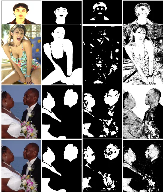
Skin detection results. (a) input image; (b) ground truth; (c) U-Net; (d) Statistical
The first two rows are from models trained on DARK. The results of U-Net are terrible, with a lot of False Positives and False Negatives. Statistical depicts a lot of False Positives too, but at least gets the skin pixels. The small size of dataset makes it hard for the CNN model to classify correctly.
The third row features a MEDIUM on DARK case, where the hypothesis of Statistical having very few True Negatives, driving the Dprs measure high, seems confirmed. U-Net on the other hand performs a quite good classification, marking almost correctly most of the skin regions.
The last row represents a LIGHT on DARK case on the same original picture of the previous row. In this case, Statistical does a much better job, especially at predicting non-skin pixels, which may indicate that the light sub-dataset contains more images featuring sky and water labeled as non-skin pixels.
Inference Times
Inference times were measured on a i7-4770k CPU for each algorithm on the same set of images, with multiple observations performed.
Deep learning: assume one prediction is already performed before starting the observations.
Statistical: create the prediction image looping on a sequence object instead of every pixel.
| Inference time (seconds) | Improved inference time (seconds) | |
|---|---|---|
| Deep Learning | 0.826581 ± 0.043 | 0.242685 ± 0.016 |
| Statistical | 0.457534 ± 0.002 | 0.371515 ± 0.002 |
| Thresholding | 0.007717 ± 0.000 | 0.007717 ± 0.000 |
Conclusion
Conclusion
- Semantic features extraction got CNN an edge
- Rule-based method proved to be really fast but struggled on darker skin tones
- Statistical method was prone to false positives
- Involving multiple metrics debunked over-optimistic results
- Data quality is important for performance
Future Work
- Improve public data quality
- Vision transformers
- U-Nets on mobile devices [15]
Bibliography
- Ramirez, G. A., Fuentes, O., Crites Jr, S. L., Jimenez, M., & Ordonez, J. (2014). Color analysis of facial skin: Detection of emotional state. In Proceedings of the IEEE Conference on Computer Vision and Pattern Recognition Workshops (pp. 468-473).
- Low, C. C., Ong, L. Y., Koo, V. C., & Leow, M. C. (2020). Multi-audience tracking with RGB-D camera on digital signage. Heliyon, 6(9), e05107.
- Do, T. T., Zhou, Y., Zheng, H., Cheung, N. M., & Koh, D. (2014, August). Early melanoma diagnosis with mobile imaging. In 2014 36th Annual International Conference of the IEEE Engineering in Medicine and Biology Society (pp. 6752-6757). IEEE.
- Brancati, N., De Pietro, G., Frucci, M., & Gallo, L. (2017). Human skin detection through correlation rules between the YCb and YCr subspaces based on dynamic color clustering. Computer Vision and Image Understanding, 155, 33-42.
- Tarasiewicz, T., Nalepa, J., & Kawulok, M. (2020, October). Skinny: A lightweight U-net for skin detection and segmentation. In 2020 IEEE International Conference on Image Processing (ICIP) (pp. 2386-2390). IEEE.
- Chicco, D., & Jurman, G. (2020). The advantages of the Matthews correlation coefficient (MCC) over F1 score and accuracy in binary classification evaluation. BMC genomics, 21(1), 1-13.
- Zhu, Q., Wu, C. T., Cheng, K. T., & Wu, Y. L. (2004, October). An adaptive skin model and its application to objectionable image filtering. In Proceedings of the 12th annual ACM international conference on Multimedia (pp. 56-63).
- Phung, S. L., Bouzerdoum, A., & Chai, D. (2005). Skin segmentation using color pixel classification: analysis and comparison. IEEE transactions on pattern analysis and machine intelligence, 27(1), 148-154.
- Schmugge, S. J., Jayaram, S., Shin, M. C., & Tsap, L. V. (2007). Objective evaluation of approaches of skin detection using ROC analysis. Computer vision and image understanding, 108(1-2), 41-51.
- Tan, W. R., Chan, C. S., Yogarajah, P., & Condell, J. (2011). A fusion approach for efficient human skin detection. IEEE Transactions on Industrial Informatics, 8(1), 138-147.
- Sanmiguel, J. C., & Suja, S. (2013). Skin detection by dual maximization of detectors agreement for video monitoring. Pattern Recognition Letters, 34(16), 2102-2109.
- Casati, J. P. B., Moraes, D. R., & Rodrigues, E. L. L. (2013, June). SFA: A human skin image database based on FERET and AR facial images. In IX workshop de Visao Computational, Rio de Janeiro.
- Kawulok, M., Kawulok, J., Nalepa, J., & Smolka, B. (2014). Self-adaptive algorithm for segmenting skin regions. EURASIP Journal on Advances in Signal Processing, 2014(1), 1-22.
- Topiwala, A., Al-Zogbi, L., Fleiter, T., & Krieger, A. (2019, October). Adaptation and evaluation of deep learning techniques for skin segmentation on novel abdominal dataset. In 2019 IEEE 19th International Conference on Bioinformatics and Bioengineering (BIBE) (pp. 752-759). IEEE.
- Ignatov, A., Byeoung-Su, K., Timofte, R., & Pouget, A. (2021). Fast camera image denoising on mobile gpus with deep learning, mobile ai 2021 challenge: Report. In Proceedings of the IEEE/CVF Conference on Computer Vision and Pattern Recognition (pp. 2515-2524).
